1.A. Acceleration Sensor
Figure 1A-1 shows a top view of the first micromachined silicon accelerometer which was presented by Roylance (1979). A cross section of the sensor was already shown in Figure 1.3.7. The chip contains two strain gauges: one on the cantilever beam and another one on the silicon substrate. The latter does not change when an acceleration is applied and is used as reference. The cantilever beam has a length of 0.5 mm (see Figure). The length of the strain gauges is 0.8 mm (each strain gauge consists of two resistors, each with a length of 0.4 mm).
(a) Explain why the strain gauge on the cantilever beam does not extend to the end of the beam.
(b) Calculate the weight of the proof mass m. The dimensions of the proof mass are 1mm x 1.2mm x 0.5mm. The density of silicon is 2330 kg/m3.
We will now simplify our calculations by assuming that the cantilever beam is loaded by a point force at its end. That is, we assume that an acceleration a results in a point force ma acting on the end of the cantilever beam. In fact this corresponds to the situation that the centre of mass of the proof mass coincides with the end of the cantilever beam.
(c) Can you explain why this is a rather rough approximation?
(d) Calculate the spring constant of the cantilever beam. The dimensions of the beam are 0.5mm (length) x 0.2mm (width) x 0.5mm (thickness).
(e) Calculate the relative change in resistance of the strain gauge on the cantilever beam as a function of the force.
(f) Calculate the resonance frequency based on the mass and spring constant calculated in (b) and (d).
(g) The strain gauges are connected as one half of a Wheatstone bridge. The other half of the bridge consists of two identical resistors. Calculate the sensitivity of the accelerometer in mV/(m/s2).
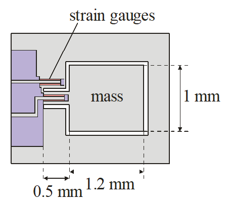
Figure 1A-1: Top view of the silicon accelerometer realized by Roylance (1979).
6.B. Compression type load cell
Figure 1B-1 shows a typical compression type load cell. Inside the load cell are 4 stainless steel columns that carry the load. Each column has 4 strain gauges (one on each side) attached to it, two of them oriented in the vertical direction, and the other two oriented in the horizontal direction. As a result, when a weight is applied, two of these strain gauges will have an increased resistance and the other two will have a decreased resistance.
(a) Calculate the strain in the four support beams as function of the applied force F, the Young’s modulus E of the material and the width w of the beams.
(b) Calculate the relative change in resistance ΔR/R of the strain gauges as function of the applied force, the Young’s modulus of the material and the width of the beams. Assume that simple metal strain gauges are used.
The strain gauges are connected in a Wheatstone bridge as indicated in Figure 1B-2.
(c) Calculate the output voltage of the bridge as a function of the applied force.
(d) What width would you choose for the columns if the maximum load to be measured is 10000 N and the material of the columns is stainless steel (Young’s modulus 200 GPa and Yield strength 2.1 GPa)? What will be the resulting sensitivity (in V/N)?
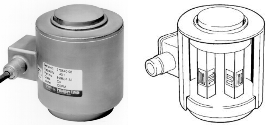
Figure 1B-1: Left: CSP-M column type strain gauge load cell from Revere Transducers. Right: Schematic drawing of the interior of such a load cell.
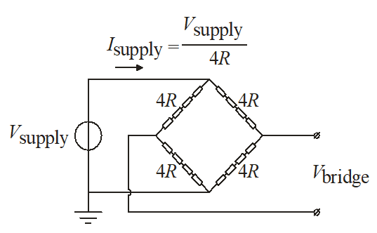
Figure 1B-2: Wheatstone bridge configuration used for readout of the load cell. The 16 strain gauges (4 strain gauges per column) are connected such that the maximum output signal is obtained.