<< Click to Display Table of Contents >> Navigation:  Part 1: Mechanical Devices > 1.2 Mechanical deformation

1.2.1. Introduction

MEMS devices typically have moving parts on a chip, which are suspended by flexures, i.e. thin strips or membranes that can deform and act like springs. Therefore, in this section an introduction is given into static mechanics and it is shown how to calculate the bending of a beam under a load. Figure 1.2.1 shows an example of a typical MEMS spring suspension, which is fabricated by SOI surface micromachining explained in Section 1.1.2. In this case the thick beams are fixed to the substrate. The 4 thin parallel beams form the spring (or flexure). This specific configuration is called a folded flexure. The moving structure is perforated, looking a bit like a brick wall that is missing the bricks. The perforation is needed so that the sacrificial layer that is underneath can be selectively etched away.

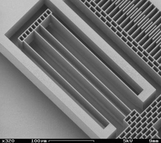
Figure 1.2.1: Scanning electron microscope (SEM) picture of a folded flexure.

In this chapter a number of Greek symbols are frequently used:

(sigma) - used to indicate stress

(epsilon) - used to indicate strain

(nu) - used to indicate the Poisson ratio

1.2.2. Types of load

We can distinguish between different types of load acting on a beam, as indicated in Figure 1.2.2. We will restrict ourselves to the cases indicated by "axial", where an axial force is applied, and "bending & shear", where a transverse force is applied.

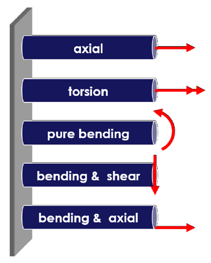
Figure 1.2.2: Different types of load. Single straight arrows indicate a force. The double arrow and the curved arrow indicates a moment.

1.2.3. Axial loads

Axial loads are relatively easy to understand. Figure 1.2.3 shows an example. A beam with cross sectional area A is loaded at the ends by an axial force F. Note that the force at each side of the beam has to be equal but opposite, for otherwise there would be a net force and the beam would start moving. Also if the beam would be fixed at one end and a force applied to the other end, there would still be an equal but opposite reaction force at the fixed end.

First we review some elementary notions for the deformation of solid bodies. We pull with a force F, which results in a stress σ given by:

The body deforms, so that it becomes longer and thinner. We have

Note that in this case ΔL is positive and Δb and Δh are negative.

The relative deformation ΔL/L is called the strain ε. For elastic materials the stress σ and strain ε are related to each other by the elasticity of the material:

where E is the Young’s modulus (also known as modulus of elasticity, elastic modulus or tensile modulus). E is a pure material property. The contraction in directions normal to the axial force is described by the Poisson ratio :

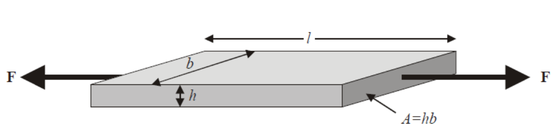
Figure 1.2.3: A beam subject to a tensile force

 

Figure 1.2.4 gives an example of a force sensor based on axial compression. The sensor chip has an area in the center that contains a large number of pillars as indicated in the cross sectional drawing. If a force F is applied on the top surface of the sensor, the pillars will be compressed and the distance between the silicon parts in between the pillars and the metal electrodes underneath will decrease, resulting in an increase in capacitance that can be measured. Suppose the pillars have an initial height h and a total combined surface area A. Then, the stress in the pillars is given by (1.1) and the strain is given by:

From this, the change in height follows:

Note that in this case the force F is negative, resulting in a negative strain and negative value of Δh.

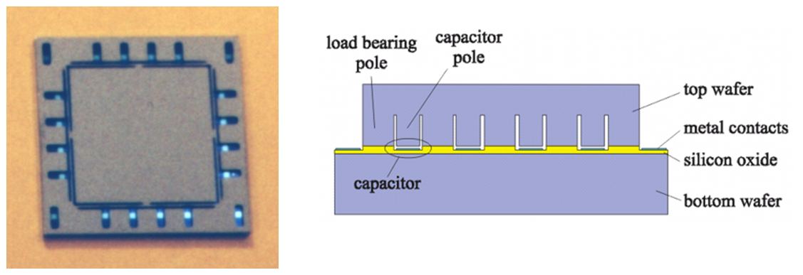
Figure 1.2.4: A silicon force sensor (also called "load cell") based on compression of pillars giving an increase in capacitance.

 

1.2.4 Transverse loads, bending of beams

We will now consider sideways or transverse forces that will result in bending of a beam. If there is a net force or moment acting on a body it will be accelerated. Thus, if a rigid body is not moving we know that there cannot be a net force or moment acting on the body, i.e.:

This must not only be true for the body as a whole, but also for each part of the body.

For example, consider the cantilever beam show in Figure 1.2.5.

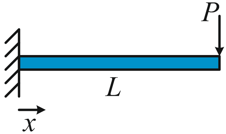
Figure 1.2.5: Cantilever beam fixed at one side and loaded by a force P at its end.

 

The net force and moment acting on this cantilever beam must be zero. Therefore, there will be reaction forces and moments at the side where it is fixed. To find these, we draw a free body diagram (FBD) as indicated in Figure 1.2.6 and apply equations (1.7) and (1.8).

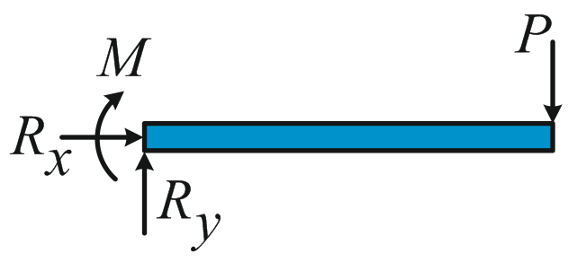
Figure 1.2.6: Free body diagram of the cantilever beam in Figure 2.

 

In principle the reaction force and reaction moment each consist of 3 components, however here we restrict ourselves to loads within the x-y plane so we only need to consider the reaction forces Rx and Ry and the reaction moment M. Applying (1.7) and (1.8), we find:

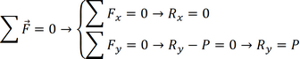
Now that we know the reaction forces and moments we can redraw the free body diagram as shown in Figure 1.2.7.

       

Figure 1.2.7: Free body diagram of the cantilever beam in Figure 2 with known reactions at the support.

 

We want to calculate the deformation of the beam, and for that we need to know the forces and moments acting inside the beam. As mentioned above, conditions (1.7) and (1.8) must also hold for parts of the body. That is, we can cut the beam in two parts at an arbitrary position x, as indicated in Figure 1.2.8, and for each part the sum of all forces and moments must be zero. This means that at the position of the cut, there must be an internal shear force V and bending moment M such that this is true. By applying (1.7) and (1.8) either to the left or right section we immediately find:

Note that the sum of moments has to be zero around any point in the x-y plane, so we can choose this point freely, at either end of the section (e.g. at the position of the cut so that the internal shear force V does not result in a moment) or elsewhere if that is more convenient.

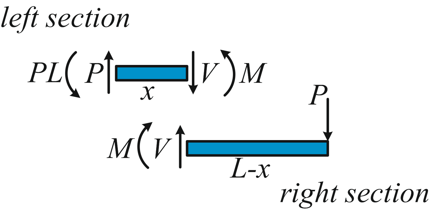
Figure 1.2.8: Free body diagrams of the left and right part of the beam when it is cut at arbitrary position x.

 

We can now draw the so-called V and M diagrams, showing the internal shear force and bending moment as a function of the position in the beam. This is done in Figure 1.2.9.

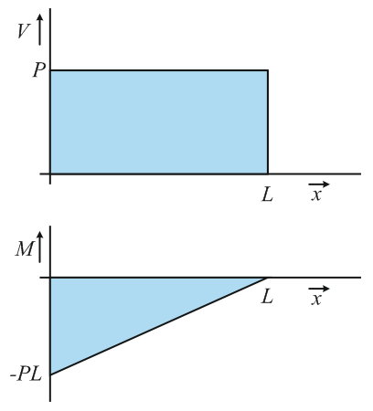
Figure 1.2.9: Internal shear force V and bending moment M diagram for the cantilever beam in Figure 1.2.5.

 

1.2.5. Finding the curvature and strain

The internal shear force and bending moment both give a deformation of the beam, however for relatively long and thin beams the effect of the bending moment is much larger and the effect of a shear deformation can be neglected. To investigate the amount of bending that results from the moment M we turn to Figure 1.2.10 which shows a segment of the beam with infinitesimal short length dx. Above the neutral line the material of the beam will be compressed. Below the neutral line the material is elongated. The amount of compression or elongation, that is the strain ε, depends on the distance y from the neutral line. We can express the strain in terms of y and the radius of curvature R:

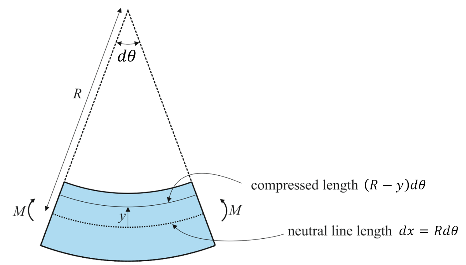
Figure 1.2.10: Beam segment with infinitesimal short length dx. The bending moment M results in a radius of curvature R.

 

Now we need to find the position of the neutral line. There is no net axial force acting on the beam, so the total force due to the compressive stress above the neutral line has to be equal to the total force due to tensile stress below the neutral line, or in other words if we integrate the stress over the cross sectional area of the beam the result should be zero:

So if we solve (1.14) we find the position that corresponds to the neutral line. Luckily, for a beam with a rectangular cross-section (or other symmetrical shapes like a circular cross-section) the neutral line will simply be in the middle.

The next step is to find the relation between the bending moment M, which we already know, and the radius of curvature R. When we know the radius of curvature we can calculate the strain using (1.13). The stress inside the beam material, compressive above the neutral line and tensile below, will result in a moment counteracting the bending moment M. For each infinitesimal small part dA of the cross-sectional area the contribution to this moment is (the minus-sign is not really important here, it defines the direction of the moment):

We know the strain from (1.13), so we can also express the stress in terms of y and R:

If we now integrate over the cross-sectional area we find the bending moment in terms of the radius of curvature:

where I is the second moment of area or area moment of inertia:

The value of I is only dependent on the cross-sectional shape. Figure 1.2.11 lists the value of I for three basic shapes.

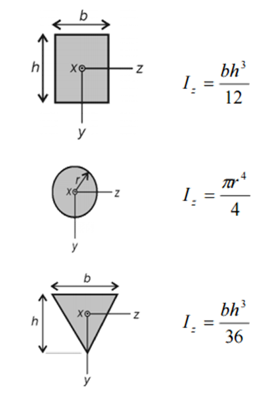
Figure 1.2.11: The second moment of area for three common cross-sectional shapes.

 

Rewriting (1.17) and inserting it in (1.13) gives us the strain as a function of the bending moment:

For the cantilever example we can now insert (1.12) to find the strain as a function of the load P and the position x along the cantilever:

So we see that the maximum strain occurs at the surface of the cantilever (maximum positive and negative value of y) at position x=0, tensile (positive) strain at the top surface and compressive (negative) strain at the bottom surface.

1.2.6. From bending radius to deflection

Equation (1.17) gives us the relation between the bending moment and the resulting radius of curvature. The next step is to find the amount of deflection or displacement of the beam with respect to its equilibrium position.

Figure 1.2.12 shows a beam with some arbitrary displacement w(x) as a function of the position x. In any point along the beam we can define the radius of curvature as indicated by the circle. We now want to relate the radius of curvature R to the displacement w(x). To this end we first note that the angle ϕ is given by:

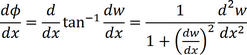
By differentiation to x we find:

Furthermore, we know the relation between an angle dϕ, the radius of curvature R and the corresponding segment dl of the beam:

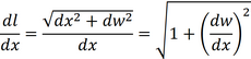
We already found the derivative dϕ/dx, so we now need to know the relation between dl and dx. For that we can express dl in terms of dx and dw, using Pythagoras’ theorem:

from which it follows that:

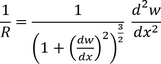
Inserting (1.22) and (1.25) into (1.23) we have found the relation between the radius of curvature R and the displacement w of the beam:

For small deflections, i.e. with dw/dx<<1, we can approximate this by:

Thus, with (1.13) we can conclude that the strain at a distance y from the center line is proportional to the second derivative of the displacement with respect to x:

Therefore, if we know the shape of the deformed structure we can use (1.28) to calculate the strain at the surface.

We can also insert (1.27) in (1.17) to find the relation between the deflection w and the bending moment M:

We can use (1.29) to find the deflection from the bending moment: we just need to integrate twice!

For the example of the cantilever beam we already found M in (1.12). Inserting (1.12) in (1.29) gives:

Integration over x gives:

With c1 an integration constant. Integrating once more we find:

With c2 another integration constant. Both integration constants c1 and c2 follow from the boundary conditions. In this case the cantilever beam is fixed at x=0. Thus, at x=0 both the deflection and its derivative will be zero:

Inserting (1.33) into (1.32) gives the deflection of the cantilever as a function of position x:

Note that for many commonly used structures it is not necessary to derive (1.34) yourself: many books provide tables with the deflections of commonly used structures at various loads. One of the best-known and most comprehensive books is “Roark's Formulas for Stress and Strain”.

To find the deflection of the tip of the cantilever we can simply insert x=L:

This also gives us the spring constant of the cantilever beam, i.e. the ratio between the applied force and the amount of displacement:

Or if we insert the second moment of area for a rectangular cross-section:

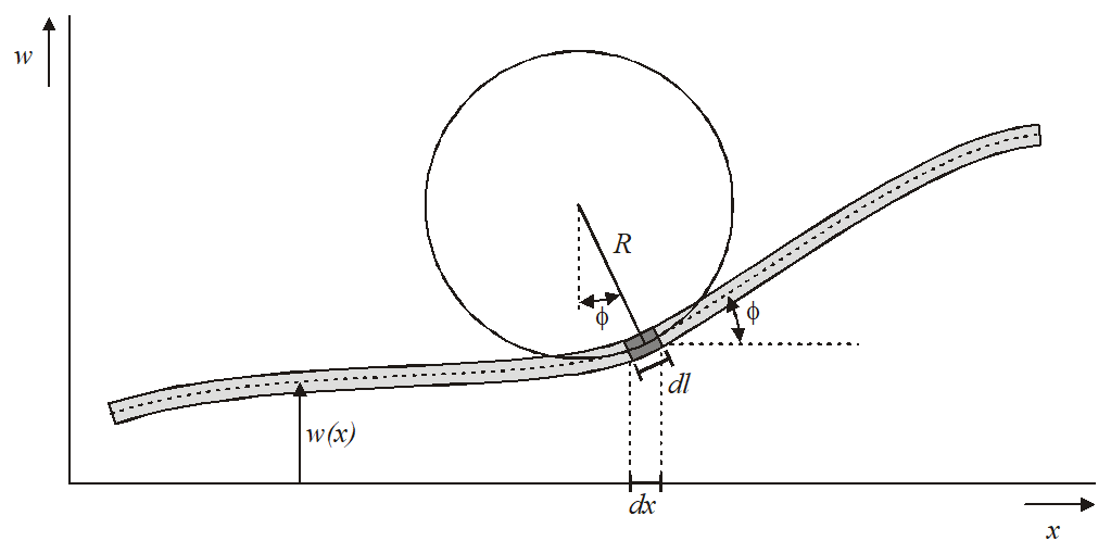
Figure 1.2.12: Relation between radius of curvature and beam displacement

1.2.7. Spring constant of a folded flexure

Now that we have found the spring constant of a simple cantilever beam in (37), we can easily extend that result to the folded flexure structure shown in Figure 1.2.1. For that we need to recognize that each of the four beams of the folded flexure can be regarded as a series connection of two cantilever beams. Furthermore, the two outer beams and the two inner beams are connected in parallel, and these pairs are connected in series again.

For two springs in parallel, the total effective spring constant is given by:

That is, the spring constants simply add up.

For two springs in series, the total effective spring constant is:

Now, try to find the spring constant of a folded flexure yourself! Assume that the four beams have a length L, a width w and a height h.

If you do the calculation correctly, you will find: